The neutrino is a type of subatomic particle. As far as we know, neutrinos are fundamental particles: that is, unlike more complicated objects like protons and neutrons, they can't be broken down into smaller constituents.
Our best current theory of particle physics, the Standard Model, contains two basic types of matter particles: hadrons, which feel the strong force that holds atomic nuclei together, and leptons, which do not feel the strong force. The most familiar lepton is the electron, which has a negative electrical charge and can therefore be detected and manipulated using the electromagnetic force. Electrons are responsible for most of the everyday properties of matter: they determine how different elements react chemically, and flows of electrons make up the electric currents that are so vital to modern technology. In the Standard Model, there are two other charged leptons, the muon (μ) and the tau (τ). Both of these are heavier than the electron and are unstable, decaying within a small fraction of a second, so they have little impact in everyday life, though they are familiar to particle physicists because they are readily created and detected in particle accelerators.
Neutrinos are leptons without electrical charge. This means that they feel only the weak force and gravity. The weak force is aptly named, and also has only a very short range (10-18 m), and gravity is unbelievably weak on the atomic scale – every time you pick something up, the electromagnetic force exerted by your muscles easily overcomes the gravitational force of the entire planet Earth – so neutrinos find it extremely difficult to "see" other particles. This makes them very hard to detect – on average, a typical neutrino could pass through a light-year of lead without interacting. They also have extremely low mass, weighing (we believe) less that one-millionth of the mass of an electron, which in turn weighs less than one-thousandth as much as a hydrogen atom. Neutrinos are therefore very elusive creatures, so much so that 25 years elapsed between the first suggestion that they must exist and the first experimental observation.
Back to Table of Contents.
To first approximation, neutrinos weigh nothing, interact with nothing and are impossible to detect. Why, then, would anyone have predicted their existence? Well, it all started with beta decay, a form of radioactive decay in which a nucleus of atomic number Z transforms to one of atomic number Z+1 and an electron is emitted. An example of beta decay is the decay of carbon-14 to nitrogen-14 used in archaeological dating: 6C14 → 7N14 + e–.
Beta decay takes place because the daughter nucleus has less mass than the parent, and therefore the decay is energetically favoured. By Einstein's E = mc2, early nuclear physicists expected that the electron would carry off the difference in masses in the form of kinetic energy. However, it turned out that the electron always carried off less energy than expected, and instead of all electrons having the same energy, there was a continuous distribution, as shown in figure 1.
|
|
| Figure 1: electron energy spectrum for beta decay of carbon-14. The red line marks the expected electron energy if only an electron were emitted. The blue line shows the observed electron energies. |
This was a very unexpected result, as energy conservation is much beloved of all physicists. At first, nobody could think of an explanation (there were even suggestions that energy conservation did not hold at the atomic level) but in December 1930 Wolfgang Pauli wrote a famous letter (translated here) to a conference in Tübingen, in which he proposed the existence of a light neutral particle of spin 1/2 emitted alongside the electron in beta decay. This explains the continuous spectrum – the available energy is split between the electron and the undetected neutral particle – and also solves a couple of more technical non-conservation problems. Pauli originally called his particle the "neutron", but when this name was given to the particle we now call the neutron (the proton-like neutral hadron discovered by James Chadwick in 1932), Fermi renamed Pauli's particle the "neutrino" (Italian for "little neutral one") – the name it still bears today.
Back to Table of Contents.
Fermi incorporated the neutrino into his ground-breaking theory of beta decay, published in 1934[1]. The success of this theory established the existence of the neutrino in the eyes of nuclear and particle physicists, but the particle itself remained elusive: indeed, Pauli worried that he might have postulated a particle which could never be detected (contrary to the principle that scientific theories should always be testable). Fortunately, the advent of nuclear fission in the 1930s and 1940s offered an unprecedentedly intense source of (anti-)neutrinos, which for the first time made the experimental detection of these elusive particles a realistic proposition.
Nuclear fission produces neutrinos because the fission of heavy elements makes isotopes that have too many neutrons to be stable. They therefore find it energetically favourable to convert the excess neutrons into protons, resulting in a cascade of beta decays. The enormous number of neutrinos produced greatly increases the chance of detecting some: as with winning the lottery, even though the chance of any given neutrino being detected (any given ticket winning the jackpot) is very small, if enough neutrinos are produced it is likely that some will be detected (if enough tickets are bought, at least one will probably win the jackpot).
During and after the Second World War, physicist Fred Reines was working at Los Alamos, involved in the testing of nuclear weapons. In 1951, as he describes in his Nobel lecture, he decided that he would like to do some fundamental physics, and after racking his brains for some months "all I could dredge up out of the subconscious was the possible utility of a bomb for the direct detection of neutrinos". Teaming up with the experimentalist Clyde Cowan, he set to work on designing the necessary detector, which would have to be very large by 1950s standards – a whole cubic metre! (In contrast, the Super-Kamiokande neutrino detector has a volume of about 50000 cubic metres.) Not only would the detector have to be very large, it would also have to be capable of surviving in close proximity to a nuclear explosion, and would have only a few seconds in which to take data before the nuclear fireball dissipated. This presented a serious technical challenge!
The reaction Reines and Cowan planned to use was inverse beta decay, νe + p → e+ + n, detected using the newly developed technology of organic liquid scintillators. This reaction produces an initial prompt burst of light when the positron annihilates with an electron to create two gamma rays (high-energy photons). The neutron bounces around for a few microseconds and is then captured by an atomic nucleus, producing another gamma ray as the nucleus releases excess energy. It was with some relief that Reines and Cowan realised that this "delayed coincidence" of two signals separated by a characteristic time lag would greatly reduce the experimental background, making it possible to use the less intense neutrino flux from a nuclear reactor instead of having to rely on a bomb.
An initial experiment at Hanford in 1953 gave tantalising hints of a signal, but was plagued by a background level much higher than expected. Tests back at Los Alamos showed that this was due to cosmic rays, and could be reduced by locating the detector underground (so that the overburden of earth absorbs many of the cosmic rays). The detector was redesigned, incorporating cadmium to improve the efficiency of neutron capture – cadmium has a very high affinity for neutrons, which is why it is used in nuclear reactor control rods. The team also relocated to the new Savannah River reactor in South Carolina, where there was an available space conveniently located 11 m from the reactor core and 12 m underground. With a more powerful reactor, a more sensitive detector, and much improved shielding from cosmic rays, the signal improved to an unambiguous 3.0±0.2 events per hour. The neutrino had finally been observed.
Back to Table of Contents.
In 1956 there were two known charged leptons, the electron and the muon (the tau was not discovered until 1975), easily distinguishable by their different masses. Each of these also had an antiparticle with opposite electric charge. Therefore, the immediate questions following the experimental observation of the neutrino were:
The first question was answered very quickly. The heavier isotope of chlorine, chlorine-37, can convert to argon-37 by inverse beta decay, ν + Cl37 → Ar37 + e–. According to the law of lepton number conservation, which states that the total number of leptons minus the total number of antileptons is always constant, this reaction must involve a neutrino (not an antineutrino); in contrast, beta decay must involve an antineutrino (because an antilepton must be produced to balance the electron). Therefore, if the neutrino and antineutrino are different, reactor neutrinos will not convert chlorine-37 to argon-37.
Ray Davis, later to become famous for his work on solar neutrinos, investigated this process using carbon tetrachloride (CCl4) as the target and the Brookhaven research reactor as the source. Over the period 1955–1960 he was able to show that the probability of this reaction was less than 10% of that expected on the assumption that the neutrino and the antineutrino were identical. This work indicated that the neutrino and antineutrino were different particles, and that the law of lepton number conservation was obeyed in weak interactions.
The second question can be answered by investigating whether the neutrinos produced in pion decays, which are always associated with a muon (the pion decays by π → μ ν, never by π → e ν) can subsequently be converted into electrons. If they can, then the two types of neutrino are not distinct. This experiment requires an accelerator, because the energies involved in radioactive decays are not nearly high enough to produce pions or muons directly.
The experiment was carried out at Brookhaven in 1962[2]. The accelerator used was the Brookhaven AGS, which produced a beam of 15 GeV protons. These protons strike a target (beryllium in this case), producing pions which are allowed to decay in flight into muons and neutrinos. A steel shield, 13.5 m thick, then absorbs all the particles except the neutrinos. The result is a beam of muon-associated neutrinos with energies up to about 1 GeV (at higher energies there is also a contribution from neutrinos produced in kaon decay, which are not guaranteed to be associated with muons).
The experiment detected 34 muon tracks, with an estimated background of 5 from cosmic-ray muons. If the neutrinos produced by pion decay were identical to those produced in beta decay, they would therefore have expected to produce about 29 electron events (they would actually see about 20, because the experiment's efficiency in detecting such events was about 2/3). If the neutrinos were different, they would expect to see perhaps one or two electrons produced by electron-associated neutrinos from kaon decays such as K+ → e+ + νe + π0. In fact, the events that were not muon-like were consistent with background from neutrons, and did not look like electrons (they had exposed their detector to a 400-MeV electron beam, so they knew what electron events should look like).
Therefore, by 1962 it appeared to be clear that neutrinos were different from antineutrinos, that neutrinos associated with electrons and muons (now called electron-neutrinos, νe, and muon-neutrinos, νμ, respectively) were different, and that the law of conservation of lepton number was obeyed separately for electrons and muons. These properties were well described by a model invented almost simultaneously by Lee and Yang, Landau, and Salam, in which the neutrinos had exactly zero mass.
Ironically, the advances in neutrino physics over the last 15 years or so have been entirely devoted to overturning all of these long-held certainties! We now know that neutrinos do have mass, and that neutrinos produced in association with electrons can subsequently interact as muon-neutrinos. We strongly suspect, but do not yet know for certain, that neutrinos and antineutrinos may not, after all, be distinct particles. This does not mean that the experiments described above were wrong, or that the Nobel Prize awarded to Leon Lederman, Mel Schwartz and Jack Steinberger for the Brookhaven two-neutrino experiment was undeserved. The masses of neutrinos are extremely tiny, and therefore the oscillation between different types (known as flavours) is very small under most experimental conditions. Similarly, the distinction between neutrinos and antineutrinos would be absolute if neutrinos were massless, and is very nearly so given that they are very nearly massless. Only very sensitive experiments, analysed with great care over many years, have allowed us to demonstrate these subtle effects.
Back to Table of Contents.
Neutrino experiments are difficult and often ground-breaking. In (sometimes long-delayed) recognition of this, a number of pioneers of neutrino physics have been awarded the Nobel Prize for Physics.
| 1988 | Leon Lederman, Melvin Schwartz, Jack Steinberger | for the neutrino beam method and the demonstration of the doublet structure of the leptons through the discovery of the muon neutrino |
| 1995 | Frederick Reines | for the detection of the neutrino |
| 2002 | Raymond Davis and Masatoshi Koshiba | for pioneering contributions to astrophysics, in particular for the detection of cosmic neutrinos |
In addition, Wolfgang Pauli (1945), Enrico Fermi (1938), and Lee and Yang (1957), who made major contributions to neutrino theory, won the Nobel Prize for work not directly connected with neutrinos. Clyde Cowan did not share in the belated prize for the discovery of the neutrino because Nobel prizes are not awarded posthumously.
Back to Table of Contents.
The principles of neutrino sources and neutrino experiments have changed remarkably little since the pioneering days of the late 1950s. In a 1960 review article[3], Fred Reines made the following points:
As a sketch of the next 50 years of neutrino physics, this has an impressive hit rate: only the study of neutrino masses by means of single and double beta decay is omitted. It is true that Reines thought that some aspects of this programme, such as the need for kiloton scale detectors, were impractical – nevertheless, it shows that the questions and challenges posed by the neutrino sector were recognised from the very beginning of the field. The results of addressing those challenges, however, have not been so predictable.
To date, artificial neutrino sources have remained very similar to those used by the pioneers. The two principal types are fission reactors, producing electron-type antineutrinos from beta decays of fission fragments, and proton accelerators, producing muon neutrinos (or antineutrinos) from pion decays in flight.
Fission reactors generate energy by breaking heavy nuclei (usually U-235) into smaller fragments. As the ratio of neutrons to protons in atomic nuclei increases as the atomic mass increases, these fission fragments have too many neutrons, and are unstable, decaying by a cascade of beta decays into stable nuclei with a lower ratio of neutrons to protons. On average, each fission yields about 200 MeV of energy and about 6 electron-type antineutrinos. It is therefore possible to estimate the number of neutrinos produced per second from the power output of the reactor.
Unfortunately, neutrino experiments need to know not just the total number of neutrinos, but also their energy distribution: the probability that a neutrino will interact in your detector depends on its energy, and the physics being studied, such as neutrino oscillations, is also energy-dependent. Calculating this is a much more difficult problem, because the original uranium nucleus can fragment in different ways producing a variety of different unstable isotopes, and additional fissionable isotopes such as plutomium-239 (produced when a neutron is captured by a nucleus of uranium-238), Pu-241 (produced when a U-238 nucleus captures several neutrons before beta-decaying to plutonium) and U-238 itself (not normally fissionable, but fission can be induced if the nucleus is struck by a fast neutron) must also be taken into account. Two techniques are employed to determine the resultant energy spectrum:
|
| Figure 2: calculated antineutrino spectra for the four main isotopes involved in nuclear reactor power generation. The spectra are normalised to one fission: in fact U-235 and Pu-239 are the dominant isotopes, with U-238 and Pu-241 together contributing about 10% of the total. Data from T.A. Mueller et al., arXiv hep-ex/1101.2663v3 |
The results of a recent calculation are shown in figure 2. The proportion of the total power that comes from U-235 and Pu-239 varies through the reactor fuel cycle, because Pu-239 is not present in the original fuel rods but is produced in the reactor itself. The spectra are all fairly similar, producing antineutrinos with energies of a few MeV. The fact that this energy is much less than the rest mass of the muon (mμc2 = 105.7 MeV) restricts the types of experiments that can be done with reactor neutrinos.
Even with all the effort that has gone into making these calculations, our understanding of these spectra remains an important contributor to the experimental error budget of experiments using reactor neutrinos. For this reason, modern reactor neutrino experiments use two detectors, a near detector close to the reactor and a far detector at a carefully selected distance (see the section on neutrino oscillations): ratios between near and far detectors can be used to study how the properties of the beam evolve with distance, and the uncertainty in the reactor neutrino flux largely cancels out.
Back to Table of Contents.
Neutrino beams from proton accelerators are produced as follows:
|
| Figure 3: the T2K neutrino beamline from the target station to the beam dump. The components of the beamline are labelled in the figure; "OTR monitor" stands for "optical transition radiation", and is used to monitor the proton beam profile immediately before it hits the target. The first horn, which surrounds the target, is used to collect positive pions; the second and third horns focus them into a collimated beam. The baffle protects the first horn from any accidental misalignment of the proton beam. |
This procedure results in a nearly pure beam of muon-neutrinos (or muon-antineutrinos if negatively charged pions are selected). The neutrino energy spectrum can be calculated from the beam parameters – this is a rather simpler task than calculating the reactor spectrum – and/or derived from the measured muon spectrum. There is some inevitable contamination with electron-neutrinos, mostly because the original pion beam also includes some kaons, which can decay to produce electron-neutrinos. Therefore, accelerator-based neutrino experiments, like reactor experiments, generally use a near detector as well as a far detector.
The energy spectrum of the neutrino beam generated in this way is rather broad: figure 4 shows the beam used by the MINOS detector at Fermilab. This can be greatly improved if the beam is deliberately offset slightly from the direction of the far detector: such an off-axis beam has a much smaller energy spread, at the cost of reduced intensity. If the proton beam is powerful enough, this is a worthwhile trade-off, and the T2K experiment uses an off-axis beam to generate a neutrino beam of comparatively well-defined energy.
|
| Figure 4: the reconstructed neutrino energy spectrum for the MINOS beam, showing the slight decrease in intensity with time, which is believed to arise from the aging of the target. Picture taken from the MINOS public plots webpage. |
Back to Table of Contents.
Although the specifications of the accelerators have improved dramatically, the above method of producing a neutrino beam from an accelerator is conceptually identical to that described by Fred Reines in his 1960 review and constructed by Lederman, Schwartz and Steinberger in their Nobel-winning 1962 experiment. All currently available neutrino beams are generated in this way, but genuinely new techniques are on the horizon for the next generation.
Beta decays generate very pure samples of electron antineutrinos (if an electron is emitted) or neutrinos (if a positron is emitted), but the energies of the neutrinos are too low for many experimental techniques: in particular, because E < mμc2, the neutrinos cannot convert to muons (and still less to the much heavier taus). The idea of the beta beam is to increase the neutrino energy by stripping the electrons off the radioactive isotope and then accelerating the positively charged ion to high energies before it decays. This boosts the energy of the neutrinos produced, and also collimates them into a fairly narrow beam. If the chosen isotope decays by electron capture (instead of emitting a positron and a neutrino, it captures one of its own orbital electrons and just emits a neutrino, e– + p → νe + n), the beam also has a very well-defined energy, although such beams are harder to make because you have to ensure that the nucleus manages to keep hold of one electron while it is being accelerated (it can't decay by electron capture if there isn't an electron to capture!).
Beta-beams have to use short-lived artificial isotopes, since a long-lived isotope such as carbon-14 would not produce enough neutrinos. Although acceleration of ions is a well-established technique (for example, the LHC has been used to collide lead nuclei), these very short-lived ions present special problems: they must be collected and accelerated quickly, before too many of them decay, and when they do decay they are lost from the beam (because their electric charge changes) and may cause the material of the accelerator to become radioactive. Radiation safety, both for the machine and for the personnel, becomes an important issue.
Although nobody has built a beta-beam so far, the technique is being intensively studied, especially at CERN, which has considerable expertise in the acceleration and storage of ions.
The ultimate accelerator-derived neutrino beam is the Neutrino Factory, which generates neutrinos by the decay of muons stored in a particle accelerator. The muons decay by μ+ → e+ νe ν͞μ: this is an extremely simple and well-understood decay and the neutrino spectra can be calculated with great precision. Although the beam is mixed, the antineutrinos are all muon-type and the neutrinos are all electron-type (swap these round if μ– are used), so they are easy to distinguish provided that your detector can determine the charge of the produced electron or muon (antineutrinos always convert to positively charged leptons and vice versa).
This is a powerful and elegant technique. The problem is that muons live for only 2.2 microseconds on average: although this is greatly extended by relativistic time dilation, even muons accelerated to 50 GeV only live for a millisecond. This means that the muons must be made, "cooled" (have their random motions reduced so that they form a nice collimated beam), accelerated and stored within a very small fraction of a second, which is a very challenging technical problem. Theoretical studies show that neutrino factories have the greatest potential for increasing our understanding of neutrinos, so this technical challenge is being addressed: for example, the Muon Ionisation Cooling Experiment (MICE) is a feasibility study aimed at showing that muons produced from pion decay can indeed be cooled into a beam suitable for acceleration and storage. However, this is still at quite an early stage, and an operational Neutrino Factory must be at least a decade away.
Back to Table of Contents.
One of the most important discoveries in neutrino physics, the phenomenon of neutrino oscillations, came about not through the use of artificial neutrino sources, but by using neutrinos produced naturally in the cosmos. Astrophysical neutrinos can provide information both on the physics of neutrinos and on important astrophysical phenomena such as supernovae and active galaxies.
|
| Figure 5: the pp chain, showing the principal branches and branching fractions. The neutrinos emitted in this series of reactions are known as pp (from the reaction at top left), Be-7 (in pp II branch), B-8 (pp III), pep (top right) and hep (centre right). Figure from [4]. |
The Sun generates energy by fusing hydrogen to helium, as first suggested by Sir Arthur Eddington as long ago as 1920. Since hydrogen contains only protons while helium has two protons and two neutrons, this process must inevitably involve the conversion of protons to neutrons, and therefore the emission of neutrinos. The process by which this is done, the pp chain, was worked out by Hans Bethe in the late 1930s, and is shown in Figure 5.
The neutrino flux from the Sun is enormous: about 60 billion per square centimetre per second. Even given the neutrino's reluctance to interact, it seems that detecting solar neutrinos should be a reasonably practical task. Unfortunately, the vast majority of solar neutrinos come from the initial deuterium production, p + p → 2H + e+ + ν (pp neutrinos), and these have very low energy, <0.42 MeV. Most methods of neutrino detection are not sensitive to such low-energy neutrinos, so most experiments rely on the higher energy Be-7 and B-8 neutrinos produced in the pp-II and pp-III side chains (the pep and hep neutrinos (see figure 5) also have high energies, but are very rare).
Solar neutrinos were first detected by Ray Davis, using the chlorine capture reaction ν + 37Cl → 37Ar + e–. This reaction is only sensitive to electron-neutrinos with energies above 0.814 MeV, so it detects primarily neutrinos from Be-7 and B-8 (see figure 6). Famously, the experiment detected only about 1/3 of the predicted number of neutrinos, thus initiating the Solar Neutrino Problem. At first, it was not clear if this was a "solar problem" (perhaps the theoretical models of the Sun's structure were not quite right), a "neutrino problem" (the theoretical model of the neutrino was not right), or an experimental problem (Davis' calculation of his efficiency in detecting Ar-37 was not right). It took many years, and many more experiments, before the second interpretation was confirmed as the correct one.
Solar neutrinos have been instrumental in studying neutrino oscillations; results from solar neutrino experiments are still a key input into calculations of neutrino mixing angles.
|
| Figure 6: energy spectrum of solar neutrinos. Most solar neutrino detectors are dominated by the Be-7 neutrinos and the B-8 neutrinos, because of their higher energies. The blue dotted lines are neutrino spectra from the CNO cycle, which contributes about 1% of the Sun's energy generation[4]. Figure from John Bahcall. |
Back to Table of Contents.
Supernovae mark the explosive deaths of stars. For a brief period, the exploding star becomes comparable in brightness to its entire host galaxy; the Galactic supernova seen in 1006 was much brighter than Venus, and was visible in daylight for weeks, despite being over 7000 light-years away. Unfortunately for astronomers, no supernovae have been seen in our Galaxy since Kepler's Supernova in 1604, but SN 1987A, a supernova observed in the Large Magellanic Cloud – a small satellite galaxy of the Milky Way, about 160000 light years away – has the distinction of being the only astrophysical object other than the Sun definitively detected as a neutrino source.
There are two main types of supernovae. Type Ia supernovae, which are extensively used by cosmologists because they all have very similar intrinsic brightness, are believed to originate in the explosive destruction of a white dwarf star which has become too massive to support itself against gravity. SNe Ia are the brightest type of supernova (SN 1006 was probably a type Ia), but are not expected to produce many neutrinos.
The other type of supernova, core-collapse supernovae (variously designated Ib, Ic, IIb, II-P and II-N depending on details of their spectra and light-curves) arise when a massive star comes to the end of its life. All stars generate energy from nuclear fusion reactions, initially using hydrogen; when the hydrogen in the central regions runs out, stars like the Sun will eventually switch to fusing helium into carbon – which requires much higher central temperatures, about 100 million kelvin as opposed to 10 million for hydrogen fusion – before dying as a white dwarf. Stars with more than 8 times the mass of the Sun can continue this process of fusing heavier elements through successively heavier isotopes, until they form a core of iron.
Iron is the most stable element: the binding energy of its nucleus is greater than the elements on either side. Elements lighter than iron can release energy by fusion; elements heavier than iron can release energy by fission; but nothing that you do to iron can release energy. As a result, once the star has formed an iron core, it is doomed. When the core becomes too massive to support itself against gravity, it collapses, and in these conditions of extreme heat and pressure the protons and electrons combine together to form neutrons, releasing electron-neutrinos. Conditions are so hot that even more neutrinos are made thermally, as neutrino-antineutrino pairs: in fact, even though to us it's the light from the supernova that is spectacular, 99% of the energy released by a core-collapse supernova comes in the form of neutrinos.
|
| Figure 7: simulation of neutrino spectra from a core-collapse supernova produced by a 15 solar mass star[5]. Solid line, νe; dashed line, νe; dotted line, all other species. In the right-hand plot, the upper lines are the luminosity and the lower lines are the mean energy. The sharp peak at t = 0 is the neutronisation pulse, when the protons in the core are converted to neutrons; the rest of the neutrinos are produced thermally. This spectrum is calculated for an observer 400 km from the collapsing core. |
Neutrinos are crucial to the understanding of core-collapse supernovae: simulations indicate that without the neutrino contribution, the star would not explode: a shock-wave is generated when the collapsing stellar envelope hits the newly formed neutron star, but it stalls in the dense medium, and is only restarted by the neutrinos. The "neutrino-driven winds" in core-collapse supernovae are also a favoured site for the so-called r-process of heavy-element building, responsible for about half the abundance of elements heavier than iron. Thus, neutrino production in core-collapse supernovae is an essential ingredient in understanding the chemical evolution of the Galaxy. Furthermore, the neutrinos come from much deeper in the stellar collapse than the light, and therefore have the potential to provide information from much closer to the initial neutron star formation.
The neutrinos from Supernova 1987A
SN 1987A was discovered just after midnight (UT) on February 24, 1987, by Ian Shelton; it was the first naked-eye supernova for nearly 400 years. Subsequent examination of earlier photographs showed that the supernova had been visible about 14 hours earlier (it was then at magnitude 6, compared to magnitude 12 for the pre-supernova star). It represented the explosion of a previously catalogued star called Sanduleak –69° 202, a blue supergiant about 20 times as massive as the Sun. This was the first time that good information, including spectra, had been available for the progenitor star of a supernova: all other modern supernovae had been observed in more distant galaxies where information on individual stars is not usually available.
The neutrino burst associated with SN 1987A was observed at 07:35:41 UT on February 23, about 3 hours before the first observation that the star had brightened in visible light (and about 5 hours after the last observation in which it definitely had not brightened). Eight neutrinos were seen by the Irvine-Michigan-Brookhaven (IMB) experiment, and 11 by the Kamiokande-II experiment (both were water Cherenkov detectors). A further 5 events were observed at the liquid scintillator Baksan detector at a time consistent with these, but this signal is much less statistically significant. An apparently significant burst observed about 4½ hours earlier by the Mont Blanc liquid scintillator detector did not correspond to a signal in any of the other detectors, and is generally assumed to have been an unlikely accidental coincidence: it is very difficult to understand two neutrino bursts 5 hours apart from the same core collapse, and nothing was seen in the larger K-II detector. (IMB had a much higher energy threshold and probably would not have seen these events.)
The neutrinos from SN 1987A generated an enormous amount of theoretical interest. From the known neutrino interaction rate and the energies of the detected neutrinos, it was possible to work out (within about a factor of 2) the amount of energy that SN 1987A must have released in neutrinos: the answer is about 3×1046 J, corresponding (using E = mc2) to a mass of 3×1029 kg. This is about 1/6 of the mass of the Sun, and confirms that most of the energy released by a core-collapse supernova is in the form of neutrinos. It is consistent with the calculated binding energy of a neutron star.
In principle, the time and energy distribution of neutrinos from a supernova could tell us a great deal about the supernova explosion, and perhaps quite a lot about neutrino physics too. The numbers detected from SN 1987A were simply too small to do very much – not that this is reflected in the huge number of theoretical papers published on the subject! – but a supernova in our Galaxy, perhaps five times closer, would produce thousands of detected neutrinos in today's larger detectors (Super-Kamiokande is 25 times the size of Kamiokande-II). We can only wait and hope!
Back to Table of Contents.
The Earth is constantly bombarded by cosmic-ray particles from space. Outside the Earth's atmosphere, these are mainly protons, with around 10–15% heavier nuclei, consistent with the general chemical composition of interstellar matter. When they hit the atmosphere, these high-energy protons interact with air molecules to produce showers of pions, which subsequently decay to muons and muon-neutrinos; some of the muons reach the ground and are detected as cosmic rays, while others decay in flight to produce more muon-neutrinos and electron-neutrinos as well. This process is exactly similar to that used to produce neutrino beams from particle accelerators. If all the muons decayed before reaching the ground, we would expect to see two muon-neutrinos for every electron-neutrino (one muon-neutrino associated with the production of the muon, one of each produced when it decays): they don't all decay, so the actual expected ratio is somewhat more than this. Early observations of atmospheric neutrinos were contradictory, with some experiments observing approximately the expected ratio while others saw significantly fewer muon-neutrinos than expected: the Atmospheric Neutrino Anomaly. After some years of disagreement, data from Super-Kamiokande finally convinced everyone that the deficit was real and a consequence of neutrino oscillations. This is generally regarded as the first definitive evidence for neutrino oscillation, although the solar neutrino experiments have some cause to feel hard done by in this.
Atmospheric neutrinos are produced with a very wide range of energies, because the primary cosmic-ray particles also have a huge energy range. Depending on your point of view, they are either an invaluable laboratory to study neutrino oscillations, or an irritating background to searches for high-energy neutrinos from astrophysical sources. Certainly, Fred Reines' 1960 opinion that atmospheric neutrinos would not be of much intrinsic interest has turned out to be unduly pessimistic!
Back to Table of Contents.
Atmospheric neutrinos are created by interactions of cosmic rays with our atmosphere – but where do the cosmic rays themselves come from? This question is not easy to answer, because cosmic rays are charged particles and therefore are deflected by the Galaxy's magnetic field as they travel through space. By the time they hit the Earth's atmosphere, their directions no longer give any information about their point of origin. Plausible theories suggest that most cosmic rays may come from supernova remnants – the expanding gas clouds left after a stellar explosion – while the most energetic examples may originate in active galaxies or gamma-ray bursts, but there is no proof of any of these hypotheses.
Whatever they are, the sources of cosmic rays are clearly accelerating protons to very high energies. It is inevitable that some of these high energy protons will collide with other particles, or with photons, within the source, generating pions and hence producing neutrinos. Therefore, every source of high-energy protons should also be a source of somewhat less high-energy neutrinos (the neutrinos carry only a fraction of the energy of the protons that produced them). These neutrinos will not be affected by the Galaxy's magnetic field, so observing them will provide clear evidence of the sites of astrophysical particle accelerators.
This is a difficult task. The number of neutrinos is small compared to the fluxes from reactors, accelerators, the Sun or Galactic supernovae, so the detectors need to be extremely large to compensate for this. In addition, the identification of muons produced by cosmic muon-neutrinos is complicated by the large background of cosmic-ray muons, and the smaller but more intractable background from atmospheric muon-neutrinos. The first background can be alleviated by looking for muons coming upwards through the Earth instead of downwards from the sky – the neutrinos will go through the Earth without difficulty, but the cosmic-ray muons will be stopped. The second is unavoidable (atmospheric neutrinos are genuine neutrinos): you just have to measure it and subtract it from any signal.
The need for very large detectors is satisfied by using natural water as a Cherenkov radiator, instead of water in tanks. The three currently operating neutrino telescopes, IceCube, ANTARES and Baikal, use Antarctic ice, the Mediterranean Sea, and Lake Baikal respectively: they are all at least 1 km underwater (or ice) to reduce cosmic-ray backgrounds, and they all look downwards, so that IceCube sees the Northern sky and ANTARES and Baikal the Southern sky. None of these experiments has yet reported a positive signal for extraterrestrial neutrinos, but so far they are limited by statistics.
Back to Table of Contents.
The nature of dark matter is one of the most intriguing unsolved mysteries of modern cosmology. A wide range of observations, from galaxy rotation curves to the structure of the cosmic microwave background, concur that about 85% of the matter in the Universe is not ordinary baryonic matter, but some exotic type of weakly interacting particle. At one time, neutrinos were themselves considered as candidates for this mysterious material, but it is now recognised that they travel too close to the speed of light to be consistent with the structure we see in the Universe (when galaxies were forming, neutrinos would be travelling too quickly for the galaxies' gravity to bind them into orbit, but observations show that the dark matter is bound in galaxies). Nevertheless, it is still possible that neutrinos may help us to solve the dark matter problem.
One of the favoured dark matter candidates is the neutralino, χ, predicted by the (as yet unconfirmed) theory of supersymmetry. If they exist, neutralinos have the right properties for dark matter: they are neutral, stable in most versions of supersymmetry, massive (probably of the order of 100 times the proton's mass) and weakly interacting. They are produced along with other particles in the very early universe, when the temperature was so high that everything had energies comparable to the beam energy of the Large Hadron Collider, and (being stable) have survived until the present day.
Neutralinos have the interesting property that they are their own antiparticle: two neutralinos can annihilate each other to produce a new particle-antiparticle pair. They cannot produce neutrino-antineutrino pairs directly, but some of the pairs they do produce (such as pairs of Z or W bosons, Higgs particles, or heavy quark-antiquark pairs) can subsequently decay to neutrinos. Therefore, neutrino production would be a possible signature of neutralino annihilation.
The snag is, of course, that as neutralinos are weakly interacting, they do not annihilate one another very easily. If the neutralinos have a mass of 150 GeV, there are something like 3000 of them per cubic metre in the vicinity of the Earth – this sounds like a lot, but it is nowhere near enough to produce a detectable annihilation rate (remember that there are 60 billion solar neutrinos per square centimetre at the Earth, and those are hard enough to detect!). Fortunately, neutralinos can be gravitationally captured by large objects like the Sun, and over time will sink into the Sun's core: theoretical calculations are inexact, because we have not discovered any supersymmetric particles yet, so we do not know what numbers to put into the equations, but they suggest that it is at least possible that neutralino annihilations in the core of the Sun could produce a detectable neutrino flux in neutrino telescopes. These neutrinos would typically have energies of a few tens to a few hundred GeV, depending on the mass of the neutralino – not as high as the neutrinos from cosmic accelerators, but far higher than neutrinos from fusion or supernova explosions. This neutrino signature would in fact be the only way to detect neutralino annihilation in the Sun's core – all the other possible annihilation products would be absorbed by the dense matter of the solar interior.
Back to Table of Contents.
We can only detect the presence of a neutrino in our experiment if it interacts. Neutrinos interact in two ways:
Charged-current interactions occur through the exchange of a W± particle, neutral-current through the exchange of a Z0.
In principle, charged-current interactions are easier to work with, because electrons and muons have characteristic signatures in particle detectors and are thus fairly easy to identify. They also have the advantage that they "flavour-tag" the neutrino: if an electron is produced, it came from an electron-neutrino. However, there must be enough available energy to allow for the mass of the lepton to be created from E = mc2 – this means that for very low-energy neutrinos (e.g. solar and reactor neutrinos) charged-current interactions are only possible for electron-neutrinos.
Various different detector technologies have been used in neutrino experiments over the years, depending on the requirements of the particular study. Desirable features of a neutrino experiment will typically include several of the following:
It is not possible to have all of these things in one experiment – for example, experiments with very low energy threshold tend not to have good angular or energy resolution. Neutrino physicists will select the most appropriate technology for the aims of their particular experiment.
The lowest energy thresholds are provided by radiochemical experiments, in which the neutrino is captured by an atom which then (through inverse beta decay, a charged-current interaction) converts into another element. The classic example of this is the chlorine solar neutrino experiment. Even lower thresholds were achieved by using gallium as the target: the reaction 71Ga + ν → 71Ge + e– has a threshold of only 0.233 MeV, and is even sensitive to pp neutrinos (see figure 6). The produced isotope is unstable, and will decay back to the original element: neutrinos are counted by extracting the product and observing these decays.
In radiochemical experiments, the target element (usually chemically bound into a compound such as C2Cl4 or GaCl3, although the SAGE experiment used pure liquid gallium) is exposed for a period comparable to the half-life of the daughter isotope. The daughter isotope is then extracted from the tank (relatively straightforward for the chlorine experiment, where the daughter is an inert gas; rather more of a challenge for the gallium experiments), and the number of radioactive decays counted. It is essential that the extraction is very efficient: typically you are trying to extract a few atoms of the product from tens of tons of the original compound!
As this brief summary of the technique makes clear, radiochemical experiments have absolutely no sensitivity to direction, cannot measure energy (beyond the simple fact that it is greater than the threshold for the reaction) and have very poor time resolution (of the order of weeks). The technique is only used in applications where a low threshold is critical – in practice, solar neutrino experiments.
Examples of radiochemical experiments: Homestake (Ray Davis; chlorine); SAGE (gallium); GALLEX/GNO (gallium).
Liquid scintillators have an impressive pedigree as neutrino detectors, since the neutrino was originally discovered using a liquid-scintillator detector. They are primarily sensitive to electron-antineutrinos, which initiate inverse beta decay of a proton: νe + p → e+ + n. Being organic compounds, liquid scintillators are rich in hydrogen nuclei which act as targets for this reaction. The positron promptly annihilates, producing two gamma rays; the neutron is captured on a nucleus after a short time (a few microseconds to a few hundred microseconds), producing another gamma-ray signal (sometimes the scintillator is loaded with an element such as gadolinium or cadmium, both of which have very high affinities for slow neutrons, to enhance this capture rate). This coincidence of a prompt signal (whose energy gives the antineutrino energy) and a delayed signal (whose energy is characteristic of the nucleus that captures the neutron – 2.2 MeV for capture on hydrogen) allows the experiment to reject background effectively.
Liquid scintillator detectors have good time and energy resolution, but do not preserve directional information. Although they are usually thought of as electron-antineutrino detectors, they are also sensitive to electron neutrinos via elastic scattering, ν + e → ν + e: the Borexino experiment uses this reaction to study the flux of B-8 solar neutrinos. They have fairly low energy thresholds, typically a few MeV, and are therefore widely used for reactor neutrino experiments.
Examples of liquid scintillator experiments: Borexino (solar neutrino experiment); KamLAND (reactor neutrino oscillation experiment); MiniBooNE (accelerator neutrino oscillation experiment); SNO+ (liquid-scintillator experiment using the SNO hardware, under construction).
Tracking detectors reconstruct the path of the charged leptons produced in charged-current interactions, either by the ionisation that they cause or by the energy that they deposit. A magnetic field causes the path of the particle to be bent, allowing the momentum of the charged particle, and the sign of its charge, to be reconstructed. These detectors are best suited to higher energy neutrinos, because the distance that a particle will travel through a detector increases as its energy increases, and longer tracks are easier to reconstruct. For the same reason, they usually perform better with muons (which are penetrating particles that leave well-defined tracks) than with electrons (which produce electromagnetic showers when they travel through dense material). A shower looks different from a muon track, so tracking detectors are usually good at separating muons from electrons; their ability to distinguish electrons from photons depends on the precise nature of the detector (photons also shower in dense material, so detectors made of solid material will have trouble in separating them from electrons; gaseous detectors, in which photons and electrons don't shower, will see ionisation from electrons but not from photons, and will thus separate them easily).
Compared to other forms of neutrino detector, tracking detectors look much more similar to conventional high-energy physics experiments such as ATLAS or CMS. However, this similarity is a bit misleading. In most particle physics experiments, the interactions take place in a small, well-defined region in the middle of the experiment, which can therefore be designed with a layered structure to take advantage of this: small, high-precision tracking detectors close to the interaction point, larger, lower-precision, less expensive technologies further out. In neutrino experiments, the interaction can happen anywhere in the detector, so any design which involves multiple different technologies must allow for this.
Tracking detectors are good at distinguishing between different event topologies and reconstructing events containing multiple particles (e.g. νμ + p → μ + n + Nπ, where N ≥ 1). These are more likely to occur in higher-energy neutrino beams.
Examples of tracking detectors: MINOS (tracking calorimeter for neutrino oscillations); MINERνA (scintillator tracker for studies of neutrino interactions); ICARUS (liquid argon tracker for neutrino oscillations); T2K ND280 near detector (scintillator tracker and gaseous tracker, for characterisation of T2K beam and studies of neutrino interactions).
The detection of charged-current events from tau neutrinos is particularly challenging, because the tau decays extremely rapidly and is therefore difficult to identify cleanly. The OPERA experiment at the Gran Sasso underground laboratory and the DONUT experiment at Fermilab both addressed this by reviving the long-disused technique of nuclear emulsions.
Nuclear emulsions are simply the sensitive material of photographic film, made into a slab instead of a thin coat, and exposed to the beam. The ionisation produced by the passage of a charged particle causes chemical changes in the emulsion, which become revealed as visible tracks when the emulsion is developed. A fine-grained emulsion can provide micrometre accuracy in track positions: ideal for reconstructing the decay of an extremely short-lived particle.
Emulsions were widely used in the early days of particle physics – indeed, since the discovery of radioactivity occurred due to the fogging of a photographic plate, it could be argued that emulsions were the very first particle detectors. They fell out of fashion because:
These are cogent disadvantages, and are fatal for high-rate environments such as the LHC. For tau-neutrino experiments, they are not so serious, and the exquisite precision of emulsion tracking was considered worth the trouble: it certainly was for DONUT, which is credited with the discovery – i.e., the first direct observation – of the tau-neutrino.
It is a well-known law of nature that nothing can travel faster than light. However, this really refers to the speed of light in a vacuum. When light travels through a transparent medium such as glass or water, it is slowed to by an amount corresponding to the refractive index of the medium: water has a refractive index of 1.33 so light in water travels at 0.75c. Particles aren't affected by the refractive index, so a particle travelling at 0.99c in a vacuum will be travelling at faster than the local speed of light if it travels through water.
|
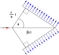
| Figure 7: the geometry of Cherenkov radiation. The particle is travelling left to right at speed βc through a medium with refractive index n. The Cherenkov cone has half-angle θ given by cos θ = 1/nβ. In many cases, the particles can be treated as extremely relativistic, β ∼ 1: in this case the opening angle depends only on the medium, cos θ = 1/n. Figure from Wikimedia Commons. |
An aircraft travelling faster than the speed of sound emits a sonic boom. Similarly, a particle travelling through a transparent medium at faster than the speed of light in that medium emits a kind of "light boom" – a coherent cone of blue light known as Cherenkov radiation. The particle is travelling down the axis of the cone, so if the cone can be reconstructed the direction of the particle can be measured.
Water Cherenkov detectors for neutrinos can be divided into two types:
Densely instrumented water Cherenkov detectors were foreseen as neutrino detectors by Fred Reines in 1960, but the pioneering IMB and Kamiokande experiments (made famous by their observations of SN 1987A) were originally conceived as detectors for proton decay. At the time, Grand Unified Theories of particle physics predicted that protons should decay (with an extremely long lifetime, of course) into e+ π0. Since the π0 immediately decays into two gamma rays, this is an ideal decay channel for water Cherenkovs, producing an easily recognisable three-ring signature. The protons failed to cooperate – the proton lifetime for this decay channel now stands at >8.2×1033 years – but the experiments proved effective in detecting solar, atmospheric and supernova neutrinos.
Water Cherenkovs can detect the electrons or muons from charged-current interactions, or the recoil electron from neutrino-electron elastic scattering. For solar neutrinos, the latter reaction dominates; for higher-energy neutrinos, the former is more important. Although it might seem that neutrino-electron scattering should be equally sensitive to all types of neutrinos, in fact it is much more sensitive to electron-neutrinos than to other types. This is because electron-neutrinos and electrons can scatter both through neutral-current interactions (the neutrino and electron retain their individual identities, but momentum is transferred from one to the other) and through charged-current interactions (the neutrino converts into an electron, and the electron converts into a neutrino). The presence of this second contribution, which is only possible for electron-neutrinos, greatly increases the chance of interaction. Therefore, water Cherenkovs are essentially electron-neutrino detectors at solar neutrino energies, but detect both electron and muon neutrinos (and flag which is which) at higher energies. (Tau neutrinos are more difficult, for two reasons: because the tau is more massive, the energy threshold above which Cherenkov radiation is emitted is much higher: 0.77 MeV for an electron, 160 MeV for a muon, 2.7 GeV for a tau; also, the tau is extremely short-lived and therefore may not travel far enough to emit much Cherenkov light.) They have good time and energy resolution, and good directional resolution for the detected particle (for low energy neutrinos, this translates into modest angular resolution for the neutrino, because the daughter particle will not be travelling in exactly the same direction as its parent).
Examples of densely instrumented water Cherenkov experiments:
Super-Kamiokande (solar neutrinos, atmospheric neutrinos, far detector for K2K and T2K
oscillation experiments); IMB (proton decay experiment, 1979–1989, which
was one of the two water Cherenkovs to detect neutrinos from SN 1987A).
Examples of neutrino telescopes: IceCube, ANTARES and
Baikal.
By the mid-1980s, the existence of the solar neutrino problem was becoming established: the theoretical model of the solar interior, the Standard Solar Model of John Bahcall and co-workers, agreed with all observations except the neutrino rate, and all attempts to find a problem with Ray Davis' experiment had failed. Over the following few years, the deficit of solar neutrinos was confirmed, first by the Kamiokande water Cherenkov experiment and then by the GALLEX and SAGE gallium experiments. It seemed overwhelmingly likely that the source of the problem lay in the behaviour of the neutrino, and specifically in neutrino oscillations. However, there was no "smoking gun": it could be proven that there was a deficit of electron-neutrinos, but it could not be shown that they had transformed into some other type of neutrino. What was needed was a detector that could directly compare charged and neutral current interaction rates at energies of order 1 MeV, far too low for muon-neutrinos to convert to charged muons.
In 1984, Herb Chen suggested that heavy water might be the solution to the problem. Heavy water, D2O, replaces normal hydrogen by its heavier isotope deuterium (2H or D), whose nucleus contains a neutron in addition to the proton of normal hydrogen. Deuterium is extremely weakly bound, and therefore easily broken up when struck; the key point is that this can happen in two different ways.
The binding energy of the deuteron is only 2.2 MeV, so any neutrino with an energy greater than this is theoretically capable of initiating the second of these reactions. The two reactions can be distinguished by detecting the capture of the neutron by an atomic nucleus – D2O is not good at capturing neutrons (which is why it's used as a moderator, to slow neutrons down in nuclear reactors without reducing the flux), but the heavy water can be loaded with some other substance to improve this (SNO used ordinary salt, NaCl; neutrons capture readily on chlorine-35).
Deuterium is a very rare isotope of hydrogen, so heavy water is expensive and difficult to obtain. Fortunately, the Canadian nuclear power industry uses heavy water in its CANDU nuclear reactors, and the SNO Collaboration was able to borrow 1000 tons from Atomic Energy of Canada Ltd. As the loan was for a fixed time, this did place a hard limit on the lifespan of the SNO experiment, which has now concluded; the vessels used to contain the heavy-water active volume and the light-water outer detector (used to reject through-going muons and other background) are being reused by the SNO+ liquid scintillator experiment.
A heavy-water Cherenkov detector is a nearly perfect experiment for low-energy neutrinos, the only drawback being that the threshold is higher than ideal for solar neutrinos (it can see only B-8 and hep neutrinos). The principal disadvantage is simply the unavailability of kilotons of D2O.
Back to Table of Contents.
The Standard Model of particle physics was developed in the mid 1970s. Over the past 35 years, it has been an extremely successful theory, providing an excellent description of most of the phenomena of particle physics. In fact, the only sector of the Standard Model that has not stood up to experimental scrutiny is its description of neutrinos.
|
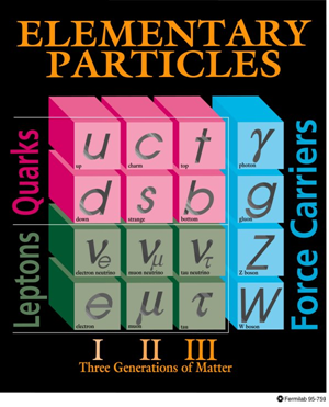
| Figure 8: the particles of the Standard Model (excluding the yet-to-be-discovered Higgs boson). Figure from Fermilab. |
At the time the Standard Model was constructed, it was assumed that:
These were the conclusions of 20 years of experimental work since the discovery of the neutrino. They were well described by the two-component model of the neutrino, which had been invented in the late 1950s by Lee and Yang, Landau, and Salam. The key ingredient of this model is the massless nature of neutrinos: if neutrinos have exactly zero mass, then their handedness (or helicity) is a permanent property, and there is no way for a neutrino created as an electron-neutrino to change into any other type. Neutrinos were the only massless matter particles in the Standard Model (photons and gluons are also massless, but they're force carriers, not matter particles) – but as masses were one of the properties that the Standard Model assumes but does not explain, this did not seem to be unreasonable.
|
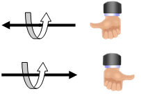
| Figure 9: helicity. Particles such as the neutrino have a property called spin, which is a quantum-mechanical version of what we normally mean by spin. The spin of a particle like a neutrino or an electron can be either right-handed, as in the top picture, or left-handed, as in the lower picture. The weak interaction selects left-handed particles and right-handed antiparticles. Note that an observer who was moving faster than the particle would see the particle's velocity change direction (if you are moving rapidly left to right, the lower particle will seem to you to be moving right to left), but its spin would remain the same – therefore its observed helicity would change. |
The handedness of a particle is only a fixed quantity, the same for all observers, if the particle has exactly zero mass (because then it will travel at the speed of light, and cannot be overtaken). Massive particles can be seen as either left-handed or right-handed depending on the motion of the observer. Therefore, if neutrinos turn out to have non-zero mass, the two-component model breaks down, and the Standard Model must be modified. It turns out that the other properties of the original model of neutrinos – the distinctness of the three flavours, and the difference between neutrinos and antineutrinos – also depend critically on the masslessness of neutrinos.
Back to Table of Contents.
With hindsight, the first crack in the foundations of the Standard Model picture of neutrinos was already visible before the model was even built. Results from Ray Davis' chlorine-37 solar neutrino experiment showed that the electron-neutrino flux from the Sun was only about 1/3 of that expected from the predictions of the Standard Solar Model. At the time, this was not taken too seriously by particle physicists, who did not have the technical knowledge to appreciate the reliability of the solar model (there was a tendency for astrophysicists to blame the neutrinos, and particle physicists to blame the astrophysics). However, in the late 1980s the reality of the deficit was confirmed by Kamiokande-II, which observed only 46(±15)% of the expected flux of high-energy solar neutrinos (>9.3 MeV), and a few years later this was joined by the GALLEX and SAGE gallium experiments, which saw about 62(±10)% of the SSM prediction for energies >0.233 MeV. Because elastic scattering preserves some directional information, K-II could demonstrate that its neutrinos really were coming from the Sun; the GALLEX and SAGE experiments calibrated their efficiency using artificial radioactive sources.
Therefore, by the mid-1990s, the Solar Neutrino Problem had become a real issue. The challenges faced by theorists attempting to explain the observations can be summarised as follows:
|
| Figure 10: the solar neutrino problem, as of the year 2000. The blue bars are measured values, with the dashed region representing the experimental error; the central coloured bar is the Standard Solar Model with its error. Each colour corresponds to a different type of neutrino, as shown in the legend. Note that because neutrino interaction probabilities depend on energy, the expected number of neutrinos detected from each process is not strictly proportional to the number produced by each process. |
Any theory seeking to explain the data would have to reproduce these features.
At first, the candidate explanations could be divided into two broad classes: either there's something wrong with the solar model, or there's something wrong with the neutrinos.
By the mid-1990s, therefore, it appeared unlikely that the Standard Solar Model could be the solution to the Solar Neutrino Problem. The technology required to explain it using neutrino properties, neutrino oscillations, had been invented as long ago as 1957, by Bruno Pontecorvo, and oscillation solutions to the problem had begun appearing in physics journals as early as 1980. However, most of the conventional particle physics community regarded solar neutrinos as an obscure corner of neutrino physics, difficult to understand and probably untrustworthy. Hence, the evidence that was seen as definitively pointing to neutrino oscillations came from another source.
Back to Table of Contents.
Meanwhile, various experiments across the world wer beginning to make measurements of atmospheric neutrinos, initially with a view to determining the background that these would present for proton decay experiments. As discussed above, atmospheric neutrinos are produced by cosmic rays impacting on the Earth's atmosphere, and should consist of muon-neutrinos and electron-neutrinos in the ratio of 2:1, or perhaps a bit more. However, experiments' efficiency for detecting and identifying muons is typically different from their efficiency for electrons, so most experiments chose to report their results as a double ratio: (muon:electron)observed/(muon:electron)predicted, where the "predicted" ratio was evaluated after simulating the detector response and passing through the whole experimental analysis chain. If the observations agreed with predictions, this ratio should be 1 within experimental error.
|
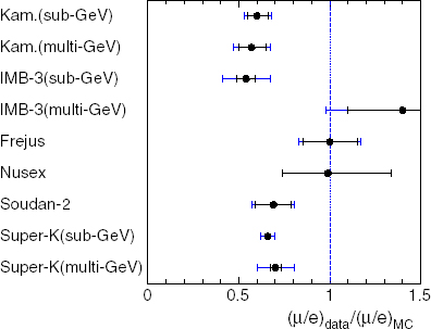
| Figure 11: compilation of results on the atmospheric neutrino anomaly, from [6]. |
Though there had been some earlier hints, useful results began to appear in the late 1980s and early 1990s. Initially, these were problematic, as shown in figure 11: water Cherenkov detectors (Kamiokande and IMB) saw anomalously low double ratios, representing a significant deficit in muon-neutrinos, while tracking calorimeters (Fréjus, NUSEX) saw no discrepancy. The coincidence that the results appeared to be correlated with detector type sparked suspicions that some kind of systematic error was involved: fortunately, by 1994 Soudan-2, a tracking calorimeter, was reporting results in line with the water Cherenkovs, lending credibility to the reality of the muon-neutrino deficit.
In 1998, Super-Kamiokande published detailed studies, using several different sub-samples of data (sub-GeV, multi-GeV, fully-contained, stopping, through-going). A striking feature of these results was the zenith angle distribution for muon-neutrinos, as shown in figure 12: the deficit occurred only in the upward-going sample, where the neutrinos had passed through the Earth before being detected. This is not caused by absorption of the neutrinos within the Earth – the interaction probability for neutrinos of this energy is far too small for that to be a problem, and no such deficit was seen for electron-neutrinos. However, if the neutrinos are oscillating from one flavour to another, the probability that a neutrino created as a muon-neutrino is observed as a muon-neutrino depends on the distance travelled, In this picture, the number of muon-neutrinos was lower for zenith angles >90° because these neutrinos had travelled a greater distance. The distribution predicted using this model, the green line, fits the data very well – as it did for all the subsamples (for example, figure 14 in [6] gives 8 separate muon zenith angle plots, all well fitted by oscillations).
|
| Figure 12: typical zenith angle ditribution, from Super-K web page. The amount by which the data fall short of the expectation (red line) increases as the distance travelled increases. |
For most members of the particle physics community, the publication of the Super-Kamiokande results marked the "discovery" of neutrino oscillations, despite the long previous history of solar neutrino measurements. The absence of any excess in the electron-neutrino sample indicated that the oscillation being observed was not νμ → νe; Super-K concluded that the best explanation was νμ → ντ, with the tau neutrinos unobserved because of the high mass and short lifetime of the tau lepton.
Back to Table of Contents.
So what are these neutrino oscillations, and how do they work?
The fundamental idea behind oscillations is the quantum-mechanical concept of mixed states, the best-known example being Schrödinger's infamous cat. In quantum mechanics, if there is a 50% chance that the cat is alive, and a 50% chance that it is dead, then until it is observed it is in a mixture of the two states. For neutrinos, the same idea can lead to oscillation. Although the neutrino is in a well-defined flavour state when it is produced (defined by the charged lepton with which it was associated), and it is in a well-defined flavour state when it interacts, it is not in a well-defined flavour state when it travels between the two. The property that is well-defined as the neutrino travels is its mass: as there are three different types of neutrino, there will be three distinct mass states – but in general these will not line up perfectly with the three different flavour states. The consequence of a mismatch is as follows:
The mathematics of oscillation is essentially identical to the mathematics of rotation. If only two flavours and two masses are involved, the rotation can be described by a single angle θ – for three flavours, three angles are required, and the mathematics becomes much more complicated.
|
| Figure 13: rotating coordinate axes. The black axes represent the flavour states: the black star marks a neutrino in a pure electron-neutrino state. The red axes, rotated by an angle θ, represent the mass states. Note that the black neutrino is not in a pure mass state: it contains a mixture of both masses. The red star is a neutrino in a pure mass state, but it is a mixture of flavours. When it interacts, it is not certain whether it will do so as an electron-neutrino or a muon-neutrino. |
For the two-flavour case, it is fairly simple to work out the probability P that a neutrino produced as flavour α will be observed as flavour β: it is
P(α→β) = sin2(2θ) sin2(1.267 Δm2 L/E)
where θ is the mixing angle, Δm2 is the difference in the squares of the masses, m22 – m12, in (eV)2, L is the distance travelled in km, E is the energy in GeV, and 1.267 is a constant put in to make the units come out right. The important thing to notice about this formula is that θ and Δm2 are properties of the neutrinos, but L and E are properties of the experiment. The important number for a neutrino experiment is therefore the ratio L/E: if your beam energy is twice that of your rivals, you can make the same measurement by putting your detector twice as far away (or, if you already have a detector that is a known distance away, you can design your neutrino beam to make best use of it by adjusting E – this is what we did in T2K).
The simple two-flavour oscillation worked well to explain the atmospheric neutrino anomaly. The solar neutrino deficit, however, presented more difficulty. The problem is as follows:
The solution to this problem turned out to lie in the fact that solar neutrinos are produced, not in the near-vacuum of the upper atmosphere or a particle accelerator, but in the ultradense matter of the Sun's core. In this dense material, electron-neutrinos tend to interact with the many free electrons present in the hot, dense plasma deep in the Sun. There aren't any free muons or taus, so the other neutrinos are not affected. This difference turns out to change the effective parameters of the oscillation, a phenomenon known as the MSW effect after the initials of the three theorists who first worked it out – the Russians Mikheyev and Smirnov, and the American Wolfenstein.
|
| Figure 14: neutrino fluxes from SNO. The x-axis shows electron-neutrino flux, the y-axis flux of other neutrinos (it is not possible to distinguish μ and τ). The red band shows the result of the charged-current analysis, sensitive to electron-neutrinos only; the blue band is the neutral-current analysis, equally sensitive to all types. The green band is elastic νe scattering, which prefers electron-neutrinos but has some sensitivity to other types, and the brown band is the higher-precision result on this from Super-K. The band between the dotted lines is the total neutrino flux expected in the Standard Solar Model. |
The key feature of the MSW effect is that under certain conditions it is resonant – it efficiently converts all electron-neutrinos into some other type. For the Sun, the low-energy neutrinos produced in the pp reaction are almost unaffected, whereas higher energy neutrinos hit the resonance: this accounts for the apparent near-total disappearance of the Be-7 neutrinos. A feature of the resonance is that it only happens if the mass state that is mostly electron-neutrino is lighter (in a vacuum) than the one it transforms into – thus we know that the mostly-electron-neutrino mass state is not the heaviest of the three. In contrast, "ordinary" oscillations, taking place in a vacuum, don't tell us which of the two states is heavier.
This explanation of the solar neutrino deficit was dramatically confirmed a few years later by the SNO heavy-water experiment, which used dissociation of deuterium to compare charged-current and neutral-current neutrino interaction rates directly. As seen in Figure 14, their results clearly show that the "missing" solar neutrinos are not missing at all: they have simply transformed into some other type. This is definitive evidence in favour of neutrino oscillations.
Back to Table of Contents.
The probability that neutrino type α transfroms into type β is zero if Δm2 = 0: if neutrinos were massless, or indeed if they all had the same mass, they could not oscillate. This is because, however you label the neutrinos, the total number of distinguishable types must remain the same, i.e. three. If there aren't three different masses, mass isn't a valid labelling scheme, so the neutrinos' identities must be defined by their interactions and there is no oscillation. This is very like locating a place on a map: you can use longitude and latitude, or Ordnance Survey map references, or a distance and bearing from a reference point ("5 km northeast of the railway station"), but you always need two numbers (three, if you also want to specify height above sea level).
|
| Figure 15: Δm2 and θ for the solar neutrino oscillation. This is the best combined fit to the solar neutrino data and the KamLAND reactor neutrino data, from [7] |
By counting the number of neutrinos they observe, experimenters can find values for the unknown Δm2 and θ in the equation for the survival probability (L and E are known from the design of the experiment). Recent results for the solar neutrino and atmospheric neutrino oscillations are shown in figures 15 and 16. Clearly the parameters are not the same, but this is to be expected: in the case of solar neutrinos we start with νe and end with something else, whereas for atmospheric neutrinos we start with νμ and end with ντ, so we are looking at different systems. It is usual to call the solar neutrino mixing θ12 and the atmospheric mixing θ23.
Because the oscillation is only sensitive to the difference in the squared masses, these results tell us that the masses are not zero, but don't tell us what they are. The squared mass difference of 8×10⁻⁵ eV2 between mass 1 and mass 2 could correspond to 0 and 0.009 eV, 0.01 and 0.0134 eV, 0.1 and 0.1004 eV, or even 10 and 10.000004 eV – the oscillation results do not tell us. For the atmospheric neutrinos, we don't even know which state is heavier. This gives us two possible ways to combine the two values of Δm2:
Normal Hierarchy: ν1 ← 8×10⁻⁵ → ν2
← 2.3×10⁻³ → ν3;
Inverted Hierarchy: ν3 ← 2.3×10⁻³ →
ν1 ← 8×10⁻⁵ → ν2.
|
| Figure 16: Δm2 and θ for the atmospheric neutrino oscillation. This plot shows both atmospheric neutrino data from Super-Kamiokande and accelerator neutrino data from MINOS, from [8] |
We know from the solar data that mass state 1 is mostly electron-neutrino, so the "normal hierarchy" is so called because it assumes that the lightest neutrino corresponds to the lightest charged lepton. Figure 16 shows that the mixing between νμ and ντ is pretty much as large as it could possibly be (θ23 ∼ 45°), so it doesn't really make sense to assign mass states 2 and 3 to "μ" and "τ" – they contain equal amounts of each.
The next generation of neutrino oscillation experiments should be able to work out the ordering of the mass states, and will improve the precision with which we know the mass splittings. To measure the masses themselves, we need to go back to the original inspiration for the idea of the neutrino – beta decay.
In beta decay, the available energy (the difference between the masses of the radioactive parent nucleus and its daughter) is shared between the electron and the neutrino. The electron, however, must get at least mec2, because its energy must be at least enough to create its own mass. If the neutrino had exactly zero mass, it could be very unlucky and get zero energy. However, we now know that neutrinos are not massless, so we have to allow the neutrino to carry away at least mνc2. This slightly reduces the maximum possible energy that could be given to the electron, so the distribution of electron energies will be modified slightly near its endpoint.
Unfortunately, it is very unlikely that the energy split between the electron and the neutrino should be so one-sided, so regardless of the isotope we choose, the number of decays in this region of the electron energy spectrum will be very small. Furthermore, because we expect that the neutrino mass is extremely small, we will need to measure the electron energy with very high precision: a small experimental uncertainty could easily wipe out our signal. Electrons are charged, so their energy is affected by electric fields – the eV unit of energy is just the energy an electron gains from a voltage drop of one volt – so if our experiment uses electric fields we need to be very careful to ensure that they do not affect the electron energies we are trying to measure. If the isotope in the experiment is in the form of a chemical compound, even the electric fields associated with the chemical bonds may be enough to distort the results, and will need to be calculated and corrected for. In short, this is a very difficult experimental measurement, and it is not surprising that nuclear physicists have been working on it for years without success (in the sense that they have failed to detect any difference from the expectation for zero mass).
The best limits on neutrino mass from beta decay come from the decay of tritium, 3H or T, which decays to helium-3 with a half-life of 12.3 years. Tritium is a good isotope to study because:
The combination of small mass difference and short half-life is very unusual – normally, if the mass difference is very small, the half-life is very long, because the atom doesn't "gain" much by decaying. For example, the isotope rhenium-187 has an even lower maximum energy release – only 2.6 keV – but its half-life is 43 billion years! Therefore, over the years since this experiment was first tried in the 1940s, tritium has been the isotope of choice in almost every case.
So far, the best results have come from the Mainz and Troitsk tritium beta-decay experiments. These have somewhat different tritium sources – Troitsk uses gaseous tritium, Mainz uses tritium condensed on to a graphite substrate – but very similar experimental set-ups. They report very similar results: an upper limit of ∼2 eV (in other words, they saw no positive evidence for a non-zero mass, but if the mass were >2 eV they would have seen something).
The Mainz and Troitsk experiments have now been superseded by a new tritium beta-decay experiment, KATRIN, currently under construction. KATRIN is essentially a larger and more advanced evolution of the basic design used by the Mainz and Troitsk detectors, and is expected to improve on their limit by a factor of 10, to 0.2 eV. In addition, the low-energy but long-lived isotope 187Re is the basis of the MARE experiment, which hopes to achieve similar sensitivity on a lightly longer timescale. MARE solves the problem of the low decay rate of 187Re by using a very-low-temperature experimental design in which the rhenium is both source and detector (a concept similar to many of the double-beta decay experiments discussed in the next section). The rhenium can be either the pure metal – it is a superconductor, a property which can be exploited in low-temperature experiments – or incorporated in a compound, in this case AgReO4: the MARE Collaboration is exploring both technologies.
Although the rhenium technology is less mature than the tritium experiments, and will take some time to reach the goal of 0.2 eV sensitivity, it is important to have two different experiments using very different techniques attacking this difficult problem. We saw above that the solar neutrino deficit was only really taken seriously when it was confirmed by a second experiment: the field of neutrino physics has a history of false alarms which has made the community conservative in its approach to new results. Although the first experiment to report a non-zero result will eventually get the credit, recognition may well have to await confirmation by a second team.
Back to Table of Contents.
The Standard Model picture of neutrinos assumes that, as with all the other quarks and leptons, the neutrino and the antineutrino are quite distinct particles. In the other cases, this can be confirmed by their electric charges: the electron has negative charge, its antiparticle the positron has positive charge. Even in the case of the neutron, which is neutral overall, the quarks composing it have different charges (+2/3 –1/3 –1/3 for the neutron, –2/3 +1/3 +1/3 for the antineutron), and this can be confirmed by scattering experiments. Of the matter particles, as opposed to the force carriers, only the neutrino is both neutral and (as far as we know) genuinely elementary. This introduces a possible alternative to the concept of separate neutrinos and antineutrinos: what is the two particles were in fact identical, but only their spin direction differed? Because of the structure of the weak interaction, left-handed neutrinos would only interact as neutrinos, while right-handed neutrinos would interact as if they were antineutrinos. As long as their handedness remained unchanged, the two would behave as entirely different particles, even though in principle they were not.
A neutrino which behaves like this is called a Majorana neutrino, after the Italian theorist Ettore Majorana who first worked out the relevant mathematical description. If the neutrino were precisely massless, its handedness would be fixed, and there would be no meaningful distinction between the two pictures: all neutrinos would be left-handed, always, and all antineutrinos would be right-handed. But oscillations tell us that neutrinos cannot be exactly massless, and if they are not, then their handedness is not an unchangeable constant. Therefore, if neutrinos really are Majorana particles, it is possible in principle (if very improbable in practice, because their masses are so small), that a particle produced as a neutrino might be capable of subsequently interacting as an antineutrino. This behaviour might be seen in a very rare kind of radioactive decay called double beta decay.
Ordinary beta decay takes place when an atom converts a neutron to a proton (emitting an electron and increasing its atomic number by 1) or a proton to a neutron (emitting a positron and decreasing its atomic number by 1). This happens when the neighbouring isobar (atomic nuclei with the same atomic mass, i.e. the same total number of protons and neutrons, are called isobars) is more tightly bound, and hence has less mass, than the one that beta-decays. Howver, in some circumstances, although both neighbouring isobars weigh more than the atom in question, one of the isobars two units away in Z weighs less. In this case, the only permitted mode of decay is double beta decay, in which the nucleus simultaneously emits two electrons (and, in the Standard Model, two neutrinos – a process known as 2νββ). This is a very improbable event, and hence the lifetimes of such isobars are much, much longer than the age of the universe – at least 1019 years. For most purposes, isotopes which can only decay by double beta decay can be regarded as stable: indeed, of the 60 or so nuclear species which could in principle decay in this way, only 11 have been observed to do so.
2νββ decay is completely consistent with the original Standard Model massless neutrinos. However, if the neutrino is a Majorana particle, a modified form of this decay is possible, in which the particle emitted as a neutrino by one of the beta decays is absorbed, as an antineutrino, by the other, producing neutrinoless double beta decay (0νββ) as in figure 17.
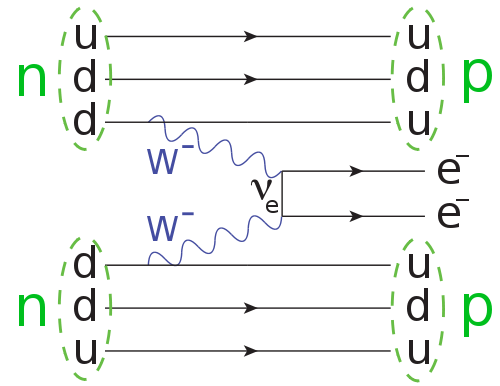
|
| Figure 17: double beta decay. Two neutrons are converted to two protons, with the emission of two electrons. The neutrino emitted by one of the decays is absorbed, as an antineutrino, by the other. Figure from Wikimedia Commons. |
Double beta decay violates lepton number conservation by 2: two electrons are produced with no corresponding antileptons. It is only possible if neutrinos are Majorana particles, so its discovery would establish the nature of the neutrino as well as a value for the mass (as we are producing electrons, the neutrino in the diagram is an electron-neutrino, so it is not a well-defined mass state: the mass we measure is a weighted average of the three possible values).
The signature of 0νββ decay is two electrons produced back-to-back, each with the same energy (corresponding to half the mass difference between the parent and daughter nuclei). In contrast, in 2νββ decay the electrons come out with a continuous energy spectrum, similar to figure 1 (in which the red line would represent the 0νββ signal). All 0νββ isotopes do of course also decay by 2νββ, so the key to a successful measurement is the ability to detect a small peak at the endpoint. And it is a small peak: lifetimes for 0νββ decay are at least 1025 years – a million times longer than the 2νββ mode.
The key requirement for a 0νββ experiment is to minimise background, since the signal is so small that even a small amount of background near the expected peak position has a serious effect on your sensitivity. The potential backgrounds include:
There are two basic techniques used in double beta decay experiments: source = detector (the isotope being measured is, or forms part of, the detector used to measure the decay) and passive source (the isotope is not part of the detector). The former type are usually cryogenic solid-state detectors measuring the ionisation produced by the decay electrons. They have good energy resolution, which is important for background suppression, and are quite small, which makes them easier to shield from environmental radioactivity. Most experiments also use the shape of the signal pulse to discriminate against background: neutrons from cosmic rays look different from electrons.
In passive-source experiments, the radioisotope is in the form of a thin film, surrounded by detector elements. These experiments usually have significantly poorer energy resolution, but can use the back-to-back topology of the emitted electrons to reduce background, since they have tracking capabilities (which the source = detector experiments generally don't). They have the advantage that they can investigate many different isotopes with the same detector (sometimes at the same time).
The double-beta decay isotope 136Xe is a special case, being a noble gas rather than a solid. It can be used, in gaseous or liquid form, as the medium for a tracking detector, similar to those used in passive-source experiments; it is also a popular candidate for ton-scale dark-matter experiments, some of which could in principle double as double-beta experiments. Unfortunately, the double-beta isotope is a relatively minor constituent (8.86%) of natural xenon, so to optimise performance the xenon has to be expensively enriched.
Most double-beta decay experiments have measured the 2νββ decay and set limits on the 0νββ decay. There is a controversial claim of a positive detection of 0νββ decay of 76Ge from the Heidelberg-Moscow experiment, corresponding to a mass of 0.4 eV (with a factor 2 uncertainty from theoretical uncertainties in the nuclear physics calculations [the nuclear matrix element]). This result is disputed, largely because there are several peaks in the endpoint region, and critics are not convinced that the one that matches the endpoint energy is not just another one of these. The GERDA experiment, using the same isotope but with higher mass and greater sensitivity, is designed to confirm or refute this disputed claim: it is currently being commissioned.
Several neutrinoless double beta decay experiments are currently operating, commissioning or under construction, all with planned sensitivities at the 0.1 eV level or better (see the Wikipedia article for a list of links). The experiments cover a wide range of isotopes, which is a good thing: the theoretical calculations of the nuclear matrix elements, necessary to predict the decay rates and to interpret any signal in terms of its implications for the neutrino mass, have large errors, and comparisons of signals from different isotopes would surely help to alleviate this. Although it seems to be easier to achieve this sensitivity in neutrinoless double beta decay than in single beta decay, we should remember that the tritium and rhenium beta-decay experiments will work for any type of neutrino, whereas the double-beta decay experiments require a Majorana neutrino.
Back to Table of Contents.
Neutrinos are extremely common in the universe: stars make them in vast numbers, and they were even more copiously produced in the first few seconds of the Big Bang. It was once thought that neutrinos with masses of order 10 eV or so might account for the dark matter, until simulations of the formation of structure in the universe showed that such fast-moving particles would produce the wrong kind of large-scale structure, making very large objects – galaxy superclusters – first, and smaller objects – galaxies – rather later (top-down structure formation). The universe we see is more consistent with a history in which galaxy-sized structures formed fast and later collected into larger systems (bottom-up structure formation), which implies fairly slow-moving, probably more massive, dark-matter particles.
However, because there are so many of them (on average, 336 per cubic centimetre everywhere in the universe, according to calculations), even the much lighter neutrinos that we currently imagine, with masses of order 0.1 eV, would contribute something to the density of the universe. This might be detected through its effect on the spectrum of temperature variations in the cosmic microwave background, as measured by WMAP (and soon by Planck). The analysis of the seven-year WMAP data sample[9] quotes a limit ∑ mν < 0.58 eV from a combined analysis of the cosmic microwave background, galaxy redshift surveys, and precision measurements of the Hubble constant. Taken at face value, this is the most stringent limit on neutrino masses currently available; it does, however, make some assumptions about the underlying cosmological model (specifically, that it has a flat geometry, and that the dark energy can be described as a cosmological constant). These are not guaranteed to hold, and therefore the quoted limit is not bullet-proof.
Supernova 1987A was also used to set neutrino mass limits. If the neutrino were massless, all neutrinos would travel at exactly the speed of light: since neutrinos aren't exactly massless, they travel more slowly than light, and their speed depends on their energy (more energetic neutrinos travel more quickly). Therefore, one would expect the more energetic neutrinos from SN 1987A to arrive here sooner than the less energetic ones, so the time distribution of the incoming neutrinos can be used to infer their masses.
This would work very well if the neutrino pulse from a supernova were instantaneous. Unfortunately, as can be seen from figure 7, it isn't, so the intrinsic time profile of the neutrino emission has to be taken into account; furthermore, the mean energy of the neutinos also evolves with time as the explosion progresses. With a large sample of neutrinos, these effects might be disentangled: with the 20 or so from SN 1987A (not all of which could safely be compared, since the Kamiokande-II and IMB clocks were not synchronised), this is not really possible, and the limits obtained were not competitive.
Back to Table of Contents.
The measurements of the "solar" and "atmospheric" oscillation parameters are now becoming quite precise (see figures 15 and 16), which means that we have to consider the full three-flavour oscillation analysis instead of assuming that only two flavours mix in any given experiment. Three flavours correspond to a three-dimensional rotation, which involves three angles (roll, pitch and yaw in the terminology of aircraft and boats), three mass differences (one of them being the sum of the other two), and one phase. The phase is the only difference between neutrino mixing and "real" rotations: it is only present if all three flavours mix, and it has a different sign for neutrinos and antineutrinos (in the terminology of particle physics, it is CP violating). This is potentially very important: one of the greatest mysteries of modern cosmology (along with dark matter and dark energy) is why the universe appears to be made up of matter, and not a 50:50 mixture of matter and antimatter, despite the fact that particles and antiparticles are usually created as particle-antiparticle pairs and have nearly identical interactions. CP-violating processes hold the key to solving this mystery.
The relationship between the three neutrino mass states (ν1, ν2, ν3) and the three flavour
states (νe, νμ, ντ) is usually expressed as a 3×3 matrix known as the PMNS
matrix after Bruno Pontecorvo, Ziro Maki, Masami Nakagawa and Shoichi Sakata. This can be written in terms of the three mixing
angles and one phase in the form
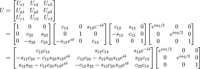
where s12 = sin(θ12), c12 = cos(θ12), δ is the CP-violating
phase, and the extra phases α1,2 only come into play in double-beta decay.
The key features of this rather forbidding-looking object are as follows:
Because Δm122 << Δm232, the difference between Δm232 and Δm132 is small, regardless of which hierarchy is correct. This means that a value of L/E appropriate to maximise the effect of θ13 will also be appropriate for θ23, which is much larger. As the atmospheric neutrino oscillation is known to involve muon-neutrinos and not electron-neutrinos, this is principally a problem for accelerator-based neutrino oscillation experiments such as T2K and MINOS. Reactor-based experiments have an electron-neutrino beam, so the relevant mass splittings Δm122 and Δm232 are well separated and L/E can be tuned to pick out one or the other.
Neutrino oscillation experiments are designed specifically to study changes in neutrino flavour – unlike the experiments that actually discovered the effect, which were just designed to detect neutrinos. There are two basic strategies:
Reactor neutrino experiments are always disappearance experiments, because the energies of reactor neutrinos – typically a few MeV – are not sufficient to create neutrinos of a different type. The only way to do an "appearance" experiment with low-energy neutrinos is direct comparison between neutral-current and charged-current reactions, as in the solar-neutrino experiment SNO. Although this was a beautiful experiment, it relied on the availability of large quantities of heavy water, which is not in general practical (SNO was a special case), so disappearance is the only realistic option.
The key issue with disappearance experiments is an accurate understanding of two things: your incoming neutrino flux (obviously, to work out how many have disappeared you need to know how many you expected in the first place) and the efficiency with which you detect events (if you are over-optimistic about this, you may think neutrinos have disappeared when in fact they were there but you missed them). The calculation of reactor fluxes is quite challenging (see our earlier discussion of artificial neutrino sources), so this has in fact been the limiting factor in some reactor experiments. If your experiment is designed to study neutrinos from one specific reactor, like Chooz, you can monitor the incoming flux by constructing two similar detectors, one close to the reactor (measuring the neutrinos before they have a chance to oscillate) and one further away: taking the ratio of the signals cancels out both the overall flux and – if the near and far detectors are of the same design – much of the uncertainty in detector efficiency. This is not so easy if, like KamLAND, you detect the combined flux from many reactors. In this case, a near detector is not really practical, although you can make some checks (if your statistics are high enough) by correlating changes in the observed flux with recorded changes in the power output of the reactors.
|
| Figure 18: oscillation in the KamLAND reactor neutrino experiment. The plot shows how the survival probability varies as a function of L/E. The points are the data (with known background subtracted); the lines are the prediction from oscillation models. From A. Gando et al., Phys. Rev. D83 (2011) 052002. |
As reactor neutrinos have quite a large energy spread, a detector at a given distance L is actually recording events at a range of values of the combination L/E which actually occurs in the oscillation equations. This means that, if your detector has good energy resolution, you can check that you are really seeing oscillation by looking for the expected sin2(1.267 Δm2 L/E) behaviour. Figure 18 shows such a plot made by the KamLAND experiment. This is an important check that the signal really is from oscillation: if it were caused by an error in the calculated flux, or by unsuspected problems in reconstructing the events, you would not expect to see this nice sinusoidal pattern.
Appearance experiments could be said to be more elegant than disappearance experiments, in that there can be no arguing with a positive result: if your initial beam was pure type X, and you see some neutrinos of type Y, something has definitely happened. In practice, the distinction is not so clear-cut: accelerator-generated muon-neutrino beams are not 100% pure (they always contain a small fraction of electron-neutrinos), and particle identification in detectors is not 100% efficient (there is a chance that you see an event of type X, but mistake it for type Y, or that you see an event which is simply background, neither X nor Y, but identify it as type Y). This sets up the key design issues for appearance experiments: you must have a good understanding of your beam, including an accurate estimate of the intrinsic contamination from other flavours, and you must have a very well-understood detector, with good particle identification, and a good knowledge of any possible background processes.
Beam characterisation requires a near detector: you measure the beam before it has a chance to oscillate, and compare these results with the results from your far detector. If the near and far detectors are very similar (the near detector perhaps scaled down to reflect the higher flux), comparing near and far detectors will also cancel out some detector effects, as with the disappearance experiments. This is the approach taken by the MINOS experiment – which is primarily a disappearance experiment, but is also designed to look for νe appearance.
In T2K, the near detector is also tasked with improving our understanding of possible background processes, by making measurements of various types of neutrino interaction for which the current world data sample isn't very good. An important example is the production of neutral pions, π0s, in neutral-current interactions, νμ + p/n → νμ + p/n + π0. The π0 decays into two photons. Photons in water Cherenkovs look almost identical to electrons, so if one of the photons is missed because it happens to have very low energy, you have an event that could easily be mistaken for an electron-neutrino charged-current interaction. For this reason, and because the detector is located so close to the accelerator that the number of events is expected to be large, the T2K near detector ND280 is not a water Cherenkov detector but a tracking detector. The advantages of this approach are expected to outweigh the disadvantages of having different efficiency calculations for near and far detectors.
In practice, appearance experiments using an accelerator-generated muon-neutrino beam are always disappearance experiments as well: because Δm232 and Δm132 are so very similar, an experiment designed to look for νe appearance (θ13) will also be sensitive to νμ disappearance, and the detector design needed for the appearance experiment (a near detector to measure intrinsic contamination of the beam, good electron-muon separation, good background rejection) is also very suited to disappearance measurements (the near detector gives you the muon-neutrino flux before oscillation, and the good particle identification and good background rejection are also useful for the disappearance analysis).
Example disappearance experiments: Double Chooz (reactor experiment, successor to
Chooz); KamLAND.
Example appearance experiments: MINOS, T2K,
OPERA (tau-neutrino appearance),
ICARUS (multi-purpose liquid argon tracking detector),
MiniBooNE.
A global fit to all data as of March 2011[10] gave the results shown in Table 1. Although none of the data used in this fit provide direct evidence for θ13 > 0, slight inconsistencies between different two-neutrino oscillation results give rise to a preference for θ13 > 0 in the fit results. The value is consistent with the result reported by T2K in June 2011.
|
| Table 1: results of global fit to oscillation experiments, from [10]. Where two numbers are given, the upper row corresponds to the normal hierarchy, in which m3 > m2 > m1, and the lower row is the inverted hierarchy, in which m2 > m1 > m3. The third mass difference is given by Δm322 = Δm312 – Δm212. If the assumptions made in the fit are valid, there is a 68% chance that the true values lie with the range given by the first column (1σ), 95% chance that they are in the range of the second column, and 99.7% for the third column. |
In the "nearly Standard Model" picture of three neutrinos with small but non-zero masses and large mixing between flavours, this is the current state of the art. It raises interesting questions: we have no idea why θ12 and θ23 are so large compared to θ13 (and compared to the mixing angles in the quark sector of the Standard Model), we don't know which hierarchy is correct, we don't know anything about δ (although, with θ13 larger than we thought it might be, we have some chance of measuring this in the next generation of oscillation experiments), and we don't know whether the neutrino and the antineutrino are the same particle or not. If this were the whole story, neutrino physics would be an interesting field for years to come. However, some results not included in this fit may prove to herald yet more surprises in the story of neutrinos.
The Standard Model has three of everything: three charge +2/3 quarks; three charge –1/3 quarks; three charged leptons; three neutrinos. It is, of course, possible that a fourth generation of quarks and leptons could exist, if it were too massive to be detected in current accelerators. However, we do definitely know that there is no fourth light neutrino, so if there is a fourth generation, it has a neutrino that is very unlike the three we know about.
With three neutrinos, there are only two independent mass differences: the third difference has to be the sum of the other two (if Joe is 2 years older than Alice, and Alice is 3 years older than Kim, we know Joe is 5 years older than Kim). Since the solar and atmospheric neutrino oscillations yield very distinct mass differences, we have accounted for all three neutrinos in the oscillation measurements discussed above.
Unfortunately, for some years there has been an unexplained result from another oscillation experiment: LSND, a short baseline (L = 30 m) oscillation experiment looking at νμ → νe, with the νμ produced by the decay of pions at rest (not in flight as is usual for accelerator-generated neutrino beams). The decay of π+ at rest produces a μ+ and a νμ, and the subsequent decay of the muon (which is also very nearly at rest) produces a νe and a νμ. Therefore, although the neutrinos produced are a mixture of electron and muon type, the antineutrinos are pure muon-type: looking for inverse beta decay, νe + p → e+ + n, is thus a sensitive appearance experiment for electron-antineutrinos. Even with a low-energy beam, the short baseline means that LSND has a rather small value of L/E, and so is sensitive to much higher values of Δm2 than those observed in solar and atmospheric oscillations. Nevertheless, this experiment observed a large excess of inverse beta decays over the calculated background, consistent with a signal from a squared mass difference of 0.05–100 eV2, which is quite inconsistent with the solar and atmospheric squared mass differences shown in Table 1.
Another experiment using neutrinos from pion decay at rest, KARMEN, found no evidence for neutrino oscillations. As the baseline of the KARMEN experiment (17 m) is slightly shorter, this null result does not completely contradict the LSND result, though it does reduce the allowable range of Δm2 to 0.05–1 eV2 (still inconsistent with the solar and atmospheric results), or 0.2–1 eV2 when constraints from other short-baseline experiments were taken into account. When these results were first announced around the turn of the millennium, the general reaction of the neutrino physics community was that one anomalous result was not enough evidence on which to base a major revision of the Standard Model, so over the next decade there was a general tendency to ignore the LSND result as probably wrong (presumably owing to some unsuspected additional background source). This tendency was strengthened in 2007 when the MiniBooNE experiment, a conventional accelerator neutrino experiment with L/E designed to explore the LSND signal region, found no evidence for νμ → νe oscillations (see figure 19).
|
| Figure 19: MiniBooNE neutrino oscillation results compared to other experiments. In this plot, the region to the right of the heavy black line is excluded by MiniBooNE; the regions to the right of the other lines are exluded by KARMEN and by the reactor experiment Bugey. The coloured regions represent the allowed region for LSND. The MiniBooNE result almost completely excludes the LSND region: there is only a very small overlap at the edge of the LSND range. Overall, the LSND result is excluded with 98% confidence (one chance in 50 that the LSND result is real). |
MiniBooNE was using neutrinos, whereas LSND and KARMEN were sensitive to antineutrinos. To remove this slight difference, MiniBooNE subsequently took data with an antineutrino beam (generating by setting the focusing horns in the beampipe to select π– instead of π+). To everyone's great surprise, these data did show an excess, with large error bars because of comparatively low statistics, but completely consistent with the original LSND result. Taken at face value, this indicates:
In addition, the MiniBooNE neutrino data showed an excess of electron-like events at low energies, inconsistent with the LSND signal and indeed inconsistent with any oscillation picture, but not explained by known backgrounds. The statistics for the antineutrino data are not sufficient to confirm or refute a similar excess in the antineutrino data.
While it is clear that more statistics are needed to confirm the excess, the apparent agreement of MiniBooNE and LSND in the antineutrino sector does suggest that something is going on, and that something cannot be incorporated into the standard three-neutrino model. So why are we sure that a fourth neutrino similar to the three we know about is not the answer, and what other possibilities exist?
|
| Figure 20: the Z line profile. The plot shows the cross-section for Z production (essentially, the number of Z bosons produced) as a function of the combined energy of the two LEP beams. The probability of producing a Z is greatly enhanced if the total energy matches the Z mass, so this scan traces out the Z width. The data shown here represent the total data set from all four of the LEP experiments combined, and the lines are the expectation for 2, 3 or 4 distinct types of neutrino. Figure from Phys. Rept. 427 (2006) 257–454. |
Neutrinos interact by the weak interaction, and that means that the carriers of the weak force, the W± and Z bosons, can decay into neutrinos: specifically, W+ → l+ + νl (where l = e, μ or τ), W– → l– + νl, and Z → νl + νl. The more distinct types of neutrino there are, the more ways the W and Z can decay, and therefore the shorter their average lifetime. In quantum mechanics, the Uncertainty Principle relates time to energy, and therefore a particle's lifetime to its mass: the shorter the lifetime, the greater the uncertainty in the mass (known as the width). Hence, if we measure the width of the Z boson, we can determine how many different types of neutrino it can decay into. This was done at the LEP Collider at CERN, the predecessor of the LHC. LEP collided electrons and positrons: since the Z can decay into e+e–, if you arrange for the total energy of the electron and positron beams to be equal to mZc2, a collider like LEP will make large numbers of Z bosons, and can therefore measure the width of the Z with great precision. The result is shown in figure 20: the data agree well with 3 neutrino species, and rule out 2 or 4 convincingly. Therefore we conclude that, if there is a fourth generation of Standard Model matter particles too heavy to be discovered in current experiments, it cannot have a neutrino light enough to be produced in Z decays. It certainly can't have a neutrino light enough to account for the LSND/MiniBooNE oscillation signal.
So, we need four neutrinos to account for three distinct and unrelated squared mass differences, but we can't have four Standard Model neutrinos because the Z width won't permit it. Does this mean that the LSND result has to be wrong?
The answer is no, because the Z width experiment counts only neutrinos that the Z can decay into. If there exist neutrinos that do not feel the weak interaction – for example, right-handed neutrinos – they would not be included in the Z width count, but they might still mix with the three known neutrinos. Such particles are called sterile neutrinos.
Although the original formulation of the Standard Model called for massless neutrinos, it could be argued that including neutrino masses simply puts neutrinos on the same footing as the other Standard Model particles, and therefore isn't really "beyond the Standard Model" physics. However, sterile neutrinos definitely are "beyond the Standard Model", and therefore there are no predictions of their properties or behaviour available. All we can do is to use existing data to infer the properties that such particles would need, and try to design future experiments to test for this.
Evidence in favour of sterile neutrinos
Evidence against sterile neutrinos
Attempting to satisfy all these constraints simultaneously turns out to be quite difficult. It is easier to get a good fit to the oscillation data if you introduce two types of sterile neutrino rather than one, but this may conflict with the nucleosynthesis data, which slightly favour one extra type of neutrino but definitely don't like two. On the other hand, it is possible that sterile neutrinos might not be produced in the early Universe as copiously as Standard Model neutrinos, so perhaps this is not a serious problem. A significant amount of CP violation is probably needed to explain the difference between the MiniBooNE neutrino and antineutrino data: this might be a good thing, because the asymmetry between matter and antimatter in the Universe needs CP-violating interactions. Because sterile neutrinos are outside the Standard Model, and not strongly connected to "standard" Beyond-Standard-Model phenomena such as supersymmetry, theorists can allow their imaginations fairly free range at this point, so the literature includes a wide variety of different scenarios, including 3+1 models (sterile neutrino is the heaviest state), 1+3 (it's the lightest state), 3+2, 2+3 and 1+3+1 (two sterile neutrinos, respectively both heavy, both light, or one of each), decaying sterile neutrinos, and many others. It is clear that more data, both cosmological and oscillation, are needed to help sort this out: Planck may help on the cosmology front, and new solar/reactor oscillation experiments such as SNO+ could provide useful constraints on the oscillation side.
T2K is a long-baseline oscillation experiment using an accelerator-generated muon-neutrino beam in an off-axis configuration. The off-axis configuration yields a neutrino beam with a much smaller range of energies than a head-on beam, at the cost of lower intensity – since the T2K beam is generated by a very high-power proton beam, the lowered intensity is a price worth paying for the narrow energy spread. The off-axis configuration also has the advantage that the electron-neutrinos that contaminate all accelerator-generated muon-neutrino beams tend to have higher energies than the muon-neutrinos, and are therefore easier to separate from the oscillation signal.
The T2K muon beam is generated by the high-power proton synchrotron at the J-PARC nuclear physics research facility in Tokai, on Japan's east coast, and the far detector is the famous Super-Kamiokande water Cherenkov detector, 295 km away in western Japan. The value of L/E for T2K is optimised for observation of the unmeasured third mixing angle θ13 (and thus, because the mass differences are so similar, automatically also for the "atmospheric" mixing angle θ23). (Because the locations of J-PARC and Super-K are fixed, L/E was optimised by adjusting E, which depends on the configuration of the focusing horns and the angle off the head-on direction, which was chosen to be 2.5°.). More detail about T2K can be found in the "About T2K" section of this website.
The original physical goals of the experiment, as set out in the 2006 T2K proposal, were
As will be apparent from the previous section, the first and third of these goals address the highest-priority questions in neutrino oscillations today: is the third angle non-zero, and do sterile neutrinos exist? The second goal is instrumental in achieving good measurements of θ13, and is also "automatic", in the sense that an experiment designed to look for electron-neutrino appearance in θ13 mixing is necessarily in the right L/E regime to study θ23 mixing, so failing to design the experiment to do so would be a wasted opportunity.
Although designed as a stand-alone experiment for solar and atmospheric neutrinos. Super-Kamiokande has many advantages as a far detector for an oscillation experiment: it is very large and already well-understood, and it has excellent electron-muon separation, good energy resolution (2.5% at 1 GeV), and good control of backgrounds, which have already been extensively studied as part of its atmospheric neutrino oscillation analyses. As a water Cherenkov, it is most suited to measuring muons, electrons and photons in relatively low-multiplicity events; also, as a non-magnetic detector it cannot measure the charge of the produced lepton, and therefore cannot directly distinguish between neutrinos and antineutrinos.
The T2K near detector, ND280, was purpose-built for the experiment. Its main goals are:
The first two goals are standard for oscillation experiment near detectors and are fairly self-explanatory. An example of the last category is the measurement of neutral-current π0 production: ν + p/n → ν + p/n + π0. The π0 decays immediately into two photons, which will be detected in Super-K as electron-like (fuzzy) Cherenkov rings. The desirable consequence of this is that, if the rate of π0 production is well understood, this sample can be used to count neutral-current events, and therefore provide information on whether any muon-neutrinos are oscillating into sterile neutrinos instead of ντ or νe. The undesirable consequence is that if one photon is not detected, either because it has extremely low energy and does not produce a reconstructable ring, or because its ring overlaps so much with the other photon's that the two are not separated, the event can be mistaken for νe appearance because the single electron-like ring looks like an electron. On both grounds, therefore, it is important to understand this reaction.
Although the March 2011 earthquake has caused an unscheduled delay in the experiment, the data collected before the earthquake have already yielded tentative indications of electron-neutrino appearance (see the KEK press release or, for technical details, the scientific paper). This is not, as yet, a definitive discovery: the probability that the apparent signal (six electron-like events on an estimated background of 1.5) represents a chance occurrence and not a real signal is only 0.7%, but physicists conduct hundreds of experiments every year, so the likelihood that one of those experiments sees something that has a 1% probability of occurring is in fact quite high. For this reason, physicists generally set the threshold for a definitive discovery at "5σ", corresponding to a chance probability of about 1 in 1.7 million. Nevertheless, the fact that this result has been obtained with only a small fraction of the intended final data sample of the experiment is extremely encouraging, and suggests that the goal of measuring the elusive third mixing angle is finally within reach.
T2K is not alone: the existing MINOS experiment, though not as sensitive to electron-neutrino appearance as T2K in the long term, has made excellent progress in the "atmospheric" mixing sector, and the American NOνA experiment, under construction and due to start data-taking in 2013, is another long-baseline off-axis experiment which will complement T2K in many respects. The Double Chooz reactor experiment, designed to measure θ13 by νe disappearance, will provide a measurement with very different systematic errors. All in all, it appears that the next decade of neutrino physics has every chance of being as interesting as the past two!